Imagine the scenario where a moving reciever is recieving pulses transmitted by a fixed reciever. At the receiver, the observed signal undergoes variations in amplitude, delay, and the number of multipath components due to mobility and scattering. The corresponding low pass equivalent of the signal recieved over a narrowband channel can be modeled as

$$\begin{equation} r(t) = c(t) * u(t), \end{equation}$$

where $*$ represents the convolution operation, $u(t)$ is the lowpass equivalent of the transmitted signal and $c(t)$ is the lowppass equiavalent of the channel given by

$$\begin{equation} c(t) = \sum_{n=0}^{N(t)} \alpha_n(t) e^{j2\pi f_c\tau_n(t) + \Phi_{D_n}(t)}, \end{equation}$$

such that $N(t)$ is the number of resolvable multipath components, $\alpha_n(t)$ and $\tau_n(t)$ are the amplitudes and delays respectively corresponding to the $n$-th path and $\Phi_{D_n}(t) = \int 2\pi f_{D_n}(t)dt$ is the doppler phase shift and $f_{D_n}(t)$ is the doppler frequency. Since the parameters $\alpha_n(t)$, $\tau_n(t)$ and $\Phi_{D_n}(t)$ associated with each resolvable multipath component change over time, they are characterized as random processes which we assume to be both stationary and ergodic. Consequently, the received signal is also a stationary and ergodic random process. Deriving the statistical properties of such a channel directly is generally intractable. Given these challenges, one of the popular models to charatcterize the temporal variations of the channel is Clarkes model which introduces the following simplistic assumptions to derive the autocorrelation function of the narrowband channel.

• Quasi-stationarity: Assuming that $\alpha_n(t)$, $\tau_n(t)$ and $f_{D_n}(t)$ are changing slowly enough such that they are constant over the time intervals of interest, we have $\alpha_n(t) \approx \alpha_n$, $\tau_n(t) \approx \tau_n$ and $f_{D_n}(t) \approx f_{D_n}$. With this assumption the Doppler phase shift becomes $\Phi_{D_n}(t) = 2\pi f_{D_n}t$. Hence, the overall phase of the $n$-th multipath component is

$$\phi_n(t) = 2\pi f_c \tau_n - 2\pi f_{D_n}t.$$

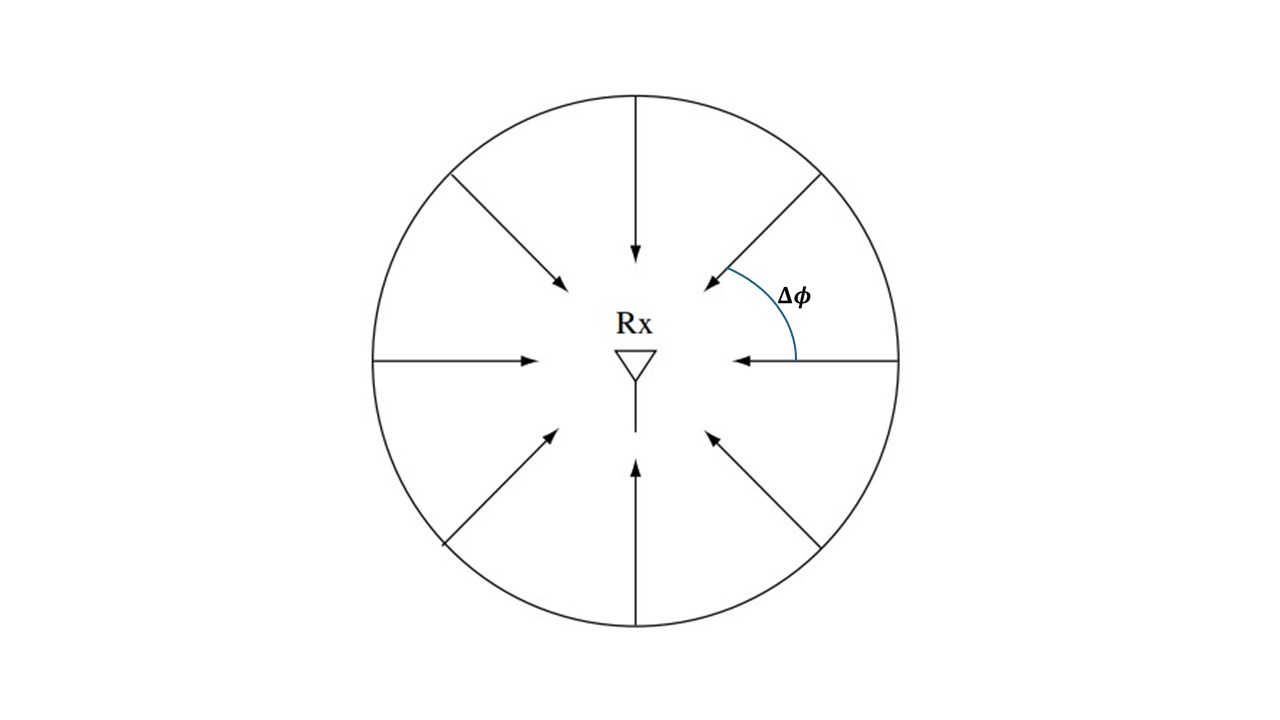
• Rapid carrier induced phase deviation: We assume that for the $n$-th multipath component the term $2\pi f_c τ_n$ in $\Phi_n(t)$ changes rapidly relative to all other phase terms. This is a reasonable assumption since $f_c$ is large and hence the term $2\pi f_c τ_n$ can go through a 360 degree rotation for a small change in multipath delay $τ_n$. Under this assumption $\Phi_n(t)$ is uniformly distributed on $[-\pi, \pi]$. Thus, it is reasonable to model the angles of arrival of $N$ multipath components as $\Phi_n = n \Delta \Phi$, where $\Delta \phi = \frac{2\pi}{N}$. This scenario is depicted in the figure below where the scatterers are places symmetrically around the reciever.

Now we move ahead to derive the various statistical properties of such a model.

Autocorrelation function (ACF) and Power spectral density (PSD) of the recieved signal

In order to characterize the ACF and PSD of the channel, we assume that the transmitted signal $u(t) = \delta(t)$. The ACF of the recieved signal can be written as

$$A_r(\tau) = E[r(t)r(t+\tau)].$$

Considering that the number of scatterers $N \rightarrow \infty$ which is realistic in rich scattering environments, the $\Delta\Phi \rightarrow 0$. In this limit, Clarke’s model yields the ACF of the received signal as

$$A_r(\tau) = P_r J_0 \left(2\pi f_D\tau\right)$$

where $J_0$ is the Bessel function of $0^{th}$ order of first kind given by

$$\begin{aligned} J_0(x) \triangleq \frac{1}{\pi} \int_0^\pi e^{-jx \cos\theta} \ d\theta \end{aligned}$$

The Bessel form reflects the isotropic scattering assumption: contributions from all directions average to this compact closed form.

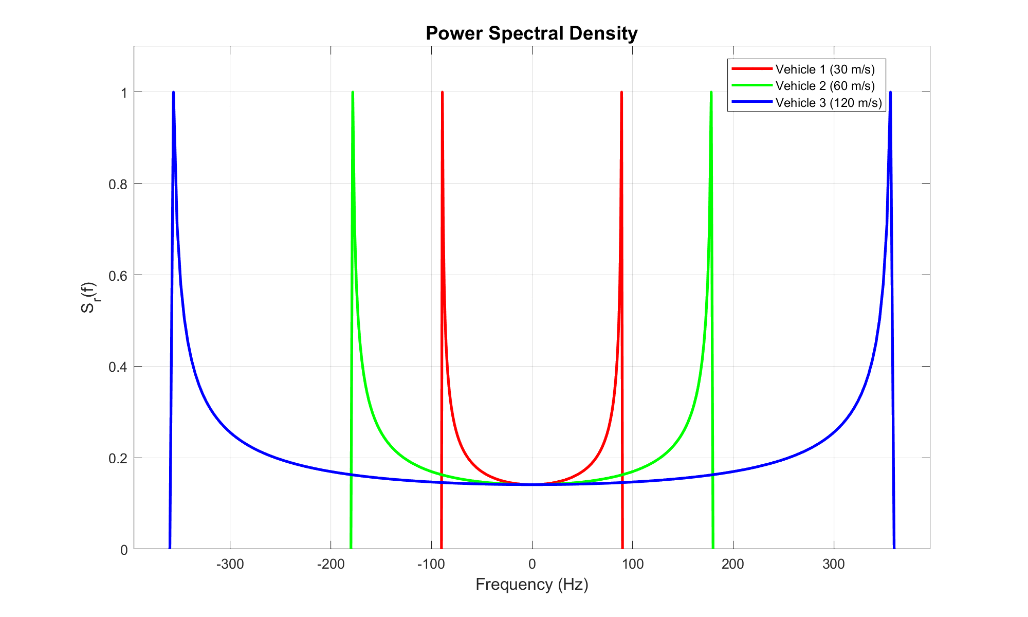
The PSD can now be obtained as usual by taking the Fourier transform of the ACF

$$\begin{aligned} S_r(f)= \begin{cases} \frac{P_r}{4\pi f_D}\frac{1}{\sqrt{1-\left(\frac{|f|}{f_D}\right)^2}} & |f| \leq f_{D} \\ 0 & \text{otherwise} \end{cases} \end{aligned}$$

where $f_D$ is the maximum doppler shift.

Impact of reciever velocity on ACF and PSD

The maximum doppler shift $f_D = \frac{v}{\lambda}$ where $v$ is the velocity of reciever and $\lambda$ is the carrier wavelength. Clearly, $f_D$ increases with velocity. This directly influences both ACF and PSD of the received signal.

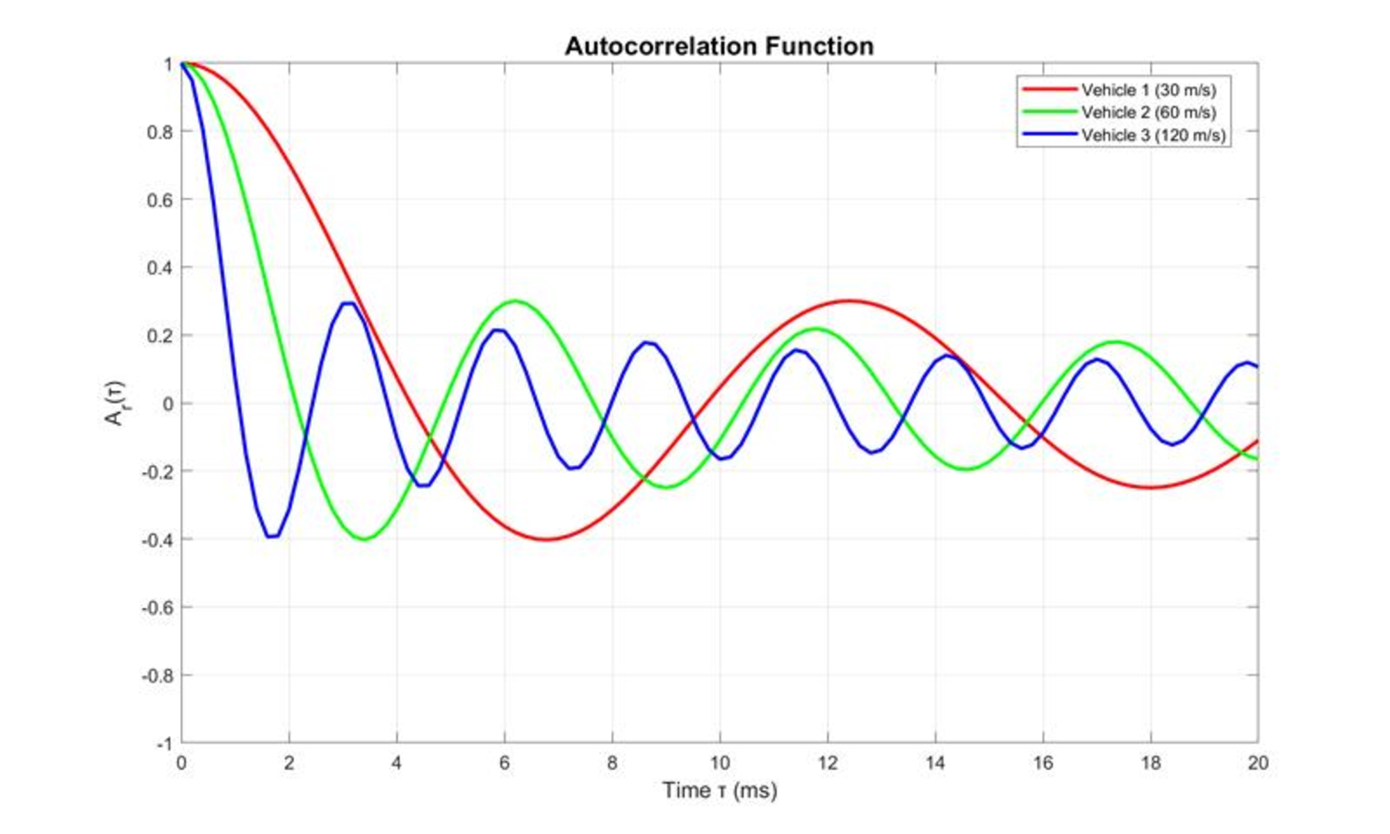
• Low velocity (small $f_D$): The oscillations of $J_0 \left(2\pi f_D\tau\right)$ are slow, and the ACF decays slowly. Thus, the channel remains correlated over a longer time (i.e. large coherence time).
• High velocity (large $f_D$): The oscillations are faster and the ACF decays quickly and the channel becomes uncorrelated in a shorter time (i.e. small coherence time).

This can be visualized in the following ACF plot wherein the red curve (correspoding to low velocity) decays slowly compared to blue curve (corresponding to higher velocity). Thus, a faster-moving receiver experiences quicker channel variations, meaning fading becomes more rapid.

The coherence time $T_c$ is the time required for the ACF to drop below a certain threshold $\alpha$ from its peak value. Using the ACF fuction, the coherence time can be expresses as

$$\begin{aligned} T_c = \frac{J_0^{-1}(\alpha)}{2\pi f_D} \end{aligned}$$

In the frequency domain, the effect of velocity appears as follows:

• Low velocity causes narrower doppler spectrum also called as doppler spread.
• High velocity causes wider doppler spectrum.

This widening of the PSD indicates stronger time selectivity (i.e. low coherence time) of the channel. This has direct implications for system design (e.g., increased inter-carrier interference in OFDM systems which are explained in the upcoming experiments). Following figure illustrates the doppler spectrum wherein the red curve shows narrower spread (correspoding to low velocity) as compared to the blue curve (correspoding to higher velocity).